 2015, Vol. 35
文章信息
- 陈春娣, 吴胜军, MeurkColinDouglas, 吕明权, 温兆飞, 姜毅, 陈吉龙
- CHEN Chundi, WU Shengjun, Meurk Colin Douglas, LÜ Mingquan, WEN Zhaofei, JIANG Yi, CHEN Jilong
- 阻力赋值对景观连接模拟的影响
- Effects of changing cost values on landscape connectivity simulation
- 生态学报, 2015, 35(22): 7367-7376
- Acta Ecologica Sinica, 2015, 35(22): 7367-7376
- http://dx.doi.org/10.5846/stxb201404010611
-
文章历史
- 收稿日期: 2014-04-01
- 网络出版日期: 2015-04-20


2. 新西兰科学院土地保护研究所, 新西兰基督城 7608
2. Landcare Research, Christchurch 7608, New Zealand
在城市化进程不断加快,自然栖息地破碎与部分生境消失不可避免的背景下,通过研究景观连接度,构建生态网络(Ecological Networks),以有限的生态用地保障城市区域生态安全[1],是当前景观生态学及空间生态学应用领域研究的热点和重点之一。景观的连接度反映了景观促进或阻碍生物体或某种生态过程在斑块间运动的程度[2],如动物迁移[3]、种子扩散[4],基因流动[5, 6, 7]等,由景观的结构特征和生物体行为特性共同决定[8, 9]。
常用的连接辨识方法包括欧氏距离(Euclidean Distance)[10],即测量斑块边缘到边缘之间的空间直线距离获得,也是斑块间的最小距离;适宜以鸟类飞行迁徙作为生态过程构建网络的研究[11]。但是对于依赖土地覆盖、下垫面属性的某些生态过程,欧氏距离则不能作为景观连接的有效度量[12, 13, 14]。相比之下,基于最小累计阻力模型(Minimum Cumulative Resistance model,MCR)的方法,即通过计算物种从源经过不同阻力的景观基质所耗费的费用或克服阻力所作的功模拟最小成本路径(Least-cost Path,LcP),则较多考虑下垫面属性以及生物体特征[10, 15, 16, 17, 18]。该模型常与景观图论理论(Landscape Graph Theory)相结合,将景观镶嵌体中的斑块、廊道等要素抽象为节点与连接[8]。通过简单、直观的图形方式来直接反映生态系统中复杂的网络结构关系,分析网络中最高效的连接路线,揭示能量、物质、基因流关系[19]。近些年在景观生态学、生物多样性保护规划中逐渐受到重视,被认为是研究景观连接,模拟网络最有效的方法[20, 21]。该方法在国外已成为以野生动物保护为目标的农田/森林栖息地质量评估或空间保护规划常用方法[22]。很多研究表明,最小成本距离比欧氏距离能够更好诠释物种在异质景观中的扩散、定居过程,以及评估景观的功能性连接度[4, 23, 24]。在国内该方法较多地应用于城市环境[25, 26],如俞孔坚等构建了北京生态安全格局[27],Kong等构建了济南城市绿网[28],Teng等运用于武汉城市绿道规划[29]。
该模型应用的关键步骤是确定阻力系数,即评估不同的土地利用/覆盖类型对物种迁移的促进或阻碍能力。理论上,阻力赋值应基于调查、观测与实验等实证研究;但是由于资金、技术和时间等限制,很多情况下,简化为土地适宜性评价结合专家经验为土地利用/覆盖类型打分,包括:(1)以植被覆盖度或植物群落多样性评价土地适宜性[28, 30]。(2)选择代理物种,如乌龟[31],刺猬[32],蝴蝶[33],通过调研文献资料获取其生活习性,评估土地阻力值。
基于MCR模型的最小成本路径辨识可在缺少观测资料的情况下,在GIS平台中较为快速地模拟斑块间连接。但在阻力面赋值时,主观性较强,如不同专家会对相同的研究区给出完全不同的阻力值[34, 35]。此外,尺度效应一直是景观生态学研究的核心问题之一[36]。众多研究表明,对景观结构特征与生态过程的度量,在不同尺度,包括幅度大小,景观粒度大小,表现不同的敏感性,产生不同的变异程度[11, 37]。尺度的选择直接关系到对景观描述与模拟的可靠性。认识模型对经验赋值及景观自身格局特征的依赖关系是有效模拟连接的前提基础。而目前较少有文献系统地研究这种效应[38],绝大部分是在具体景观中,研究某一物种运动或生态过程的连接度时,附带探讨不同赋值情况对模拟的影响[31, 39]。因此本文借鉴析因实验方法,使用一系列代表不同空间格局特征的人工模拟景观,在控制某些参数不变的前提下,比较分析不同的阻力赋值方式对景观连接模拟的影响[38],探讨、总结经验赋值所带来的不确定性与规律性,为模型应用提出一些参考建议。
1 数据与实验方法 1.1 人工景观模拟本研究的模拟景观由SIMMAP2.0 景观中性模型/软件来生成[40]。主要考虑5种决定景观格局特征的基本因子(表1),即景观幅度、斑块类型数、各类斑块优势度、空间分布方式(即景观破碎度)和景观粒度。本研究设定模拟景观幅度为300×300像元,粒度为1×1像元。因为是模拟景观,像元的面积单位可以是任意的,为便于计算与说明,假定每个像元面积单位为1m2。斑块类型的多少也即斑块丰富度。斑块优势度指某一类型斑块的面积占景观总面积的比例。本文以城市景观为依据,设定五类,即斑块类型S,A,B,C,U。S代表栖息地,即MCR模型中的源生境斑块(Source);U(Unsuitable)代表城市建筑/硬质化铺装,是最不适宜保育物种的用地类型;A,B,C则是介于最适宜与最不适宜之间的中等适宜用地类型。通常情况下,一个城市的绿地率在30%,建筑区面积在40%。排除某些高度人工化、种植单一外来物种,不适宜做源生境的绿地,本文设定S为20%;U占40%;A,B,C比例分别在5%,15%,20%。
| 景观幅度/像元Landscape extent | 斑块类型数/个Number of landscape classes | 斑块类优势度/%Dominance of classes | 景观粒度/m 2Landscape grain size | 空间分布方式Spatial distribution pattern |
| 300×300 | 5 | S: 20 A: 5 B: 15 C: 20 U: 40 | 1×1 | 聚集Clumped CP_smap=0.575 |
| 5×5 | ||||
| 10×10 | 破碎Fragmented FP_smap=0.3 | |||
| 20×20 |
空间分布方式主要指所有斑块在整个景观上的分布情况:聚集或破碎化。SIMMAP2.0中P值控制模拟景观的破碎度,取值范围在0—0.5929。值越大,景观越趋于聚集,破碎度越小。本文取2个水平,0.575与0.3分别代表聚集和破碎[41]。SIMMAP2.0是随机模拟景观,即使在参数设定完全一致的情况下,每次软件运行所生成的景观也完全是独一无二的,为了检验这种随机性是否会影响分析,本研究对变量因素及水平组合重复5次模拟。
景观粒度的变化在ArcGIS10中重采样完成。按照多数原则,即在新生成的面积单元中,以占多数像元的属性作为新像元属性,若不同属性像元数目相等时,程序随机决定新像元类型。每次重采样生成新景观时,均依据最原始的景观(即1×1分辨率的初始景观),分别产生5,10,20粒度大小的景观。各因素及水平组合后,共产生8个幅度、类型数目、斑块类优势度相同,但空间配置方式和粒度大小不同的景观,每个重复运行5次,实际上用于分析的景观共有40个(图1)。

|
| 图 1 本研究中所用模拟景观举例 Fig.1 Examples of the simulated landscapes used in this study |
最小累计阻力模型MCR和景观图论相结合在生成网络时有如下规定:①两个源斑块之间的连接不穿过其他源斑块;②连接之间没有交叉。本研究利用ArcGIS10空间分析模块和Linkage Mapper Toolist[42]插件构建景观阻力面,提取最小成本路径,其基本公式如下[15]:
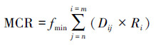
式中,MCR为物种由源扩散到空间某一点的最小累计阻力;Dij为物种从源j到景观类型i的空间距离;Ri为景观类型i对物种迁移运动阻力值,由景观基质的基本特征和物种本身的扩散能力决定;n,m为源与景观类型的数目。
1.3 阻力赋值方式对5种土地利用/覆盖类型(S,A,B,C,U)分别指定阻力值Ri。该值反映的是某一物种穿过某土地类型相比穿过栖息地S的相对难易程度[17],因为是相对值,无量纲。S为最适宜的类型,成本值最低,恒定为1;A,B,C阻力依次增加;U类型最不适宜,阻力值最大。其他类型阻力值的选取依据现有文献,主要考虑3个要素:①数值的绝对大小,如1—10,1—100,1—1000之间;②数值的相对大小,如A类型阻力值是S类型的2倍,700倍等;③类型的偏向性,包括等距赋值Ⅰ、倾向于栖息地Ⅱ、倾向于最不适宜Ⅲ、倾向于中等适宜Ⅳ,解释如表2(因整数型数值方便在GIS平台中计算,因此对于Ⅰ_a,本研究并未采用与Ⅰ_b,Ⅰ_c并列的1,2.5,5,7.5,10的赋值方式,而是采用1,2,3,4,5单独作为一种等级类型)。总共4组12个阻力赋值水平,因此,共获得480个景观阻力面(40个模拟景观×12个阻力赋值类型)。
| 赋值方式/解释Values assignment/explanation | 编号ID. | S | A | B | C | U | 赋值方式/解释Values assignment/explanation | 编号ID. | S | A | B | C | U |
| I:按照一定等级According to regulardivision | I_a | 1 | 2 | 3 | 4 | 5 | III:中等适宜地阻力赋值趋向于最不适宜Values of moderately suitable land approach to values of unsuitable land | III_a | 1 | 7 | 8 | 9 | 10 |
| I_b | 1 | 25 | 50 | 75 | 100 | III_b | 1 | 70 | 80 | 90 | 100 | ||
| I_c | 1 | 250 | 500 | 750 | 1000 | III_c | 1 | 700 | 800 | 900 | 1000 | ||
| II:中等适宜地阻力赋值趋向于栖息地,分别是1的2倍,10倍,100倍,然后按照各自最大阻力值的十分之一递增Values of moderately suitable land approach to values of habitat sources | II_a | 1 | 2 | 3 | 4 | 10 | IV:中等适宜地阻力赋值围绕最大值与最小值的平均值Values of moderately suitable land set around the mean of maximum and minimum | IV_a | 1 | 4 | 5 | 6 | 10 |
| II_b | 1 | 10 | 20 | 30 | 100 | IV_b | 1 | 40 | 50 | 60 | 100 | ||
| II_c | 1 | 100 | 200 | 300 | 1000 | IV_c | 1 | 400 | 500 | 600 | 1000 |
不同的阻力赋值可能会在空间上产生不同的最小成本路径。一般情况下,最小成本路径是曲线,其实际长度大于欧氏距离。本文构建如下公式度量最小成本路径所产生的空间偏差。
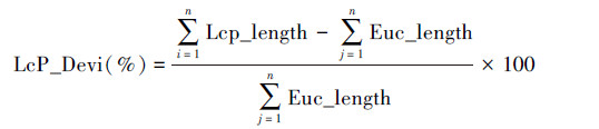
式中,Lcp_Devi表示最小成本路径空间偏差;Lcp_legth最小成本路径长度;Euc_legth欧氏距离长度;n为一个景观中模拟的最小成本路径总数量。Lcp_Devi值越大,表明某阻力赋值情景下,所产生的最小成本路径越偏离直线距离,弯曲度越大,阻力赋值对景观连接模拟的影响就越大。
2 结果空间模拟结果显示,即使在同一景观格局下,不同的阻力赋值方式会影响最小成本路径的位置(图2)。以景观粒度为1,聚集景观(P_smap=0.575)为例,赋值方式Ⅱ_a (趋向于栖息地)比Ⅲ_a(趋向于最不适宜地)的空间弯曲大,最小成本路径越偏离欧氏距离反映的景观连接方式。

|
| 图 2 不同阻力赋值下景观连接模拟举例 Fig.2 Examples of the simulated LcPs under different cost values |
每个因素及水平组合下的景观重复5次的计算结果之间没有显著差异,因此,多因素方差分析时采用每组重复的均值。表3显示了阻力赋值、空间粒度和景观破碎度对最小成本路径空间偏差的影响。3个因素分别对连接模拟产生了显著影响(P<0.001);其中,阻力赋值与粒度之间存在显著的交互作用,即阻力赋值对模拟的效应依赖于不同的空间粒度(图3和图4)。无论何种方式的阻力赋值,所反映的增长趋势基本一致,即随着粒度增大,空间偏差逐步增大,20m粒度下的平均偏差值是1m的4.2倍。并且在同一粒度下,2种破碎度水平对模拟的影响:随着景观破碎度增加,空间偏差值增大(附图)。其中直线的倾斜度表示增长程度,20 m粒度的斜率最小,表示在这一空间分辨率下,景观空间分布差异对网络模拟的影响最小。
| 来源 Source | Ⅲ型平方和Ⅲ Sum of Squares | 自由度Degree of freedom | 均方 Mean square | F | Sig. |
| R2=0.993 (修正后的R2=0.989, P<0.001) | |||||
| 阻力赋值方式Scenarios of cost values | 2004.360 | 3 | 668.120 | 119.221 | 0.000 |
| 粒度Grain size | 35677.841 | 3 | 11892.614 | 2122.155 | 0.000 |
| 破碎度 Fragmentation | 9526.740 | 1 | 9526.740 | 1699.981 | 0.000 |
| 粒度×阻力赋值方式 Grain size×Scenarios of cost values | 240.974 | 9 | 26.775 | 4.778 | 0.000 |
| 阻力赋值方式×破碎度Scenarios of cost values×Fragmentation | 5.920 | 3 | 1.973 | 0.352 | 0.788 |
| 粒度×破碎度Grain size×Fragmentation | 1290.459 | 3 | 430.153 | 76.758 | 0.000 |
| 粒度×阻力赋值方式×破碎度Grain size×Scenarios of cost values×Fragmentation | 91.167 | 9 | 10.130 | 1.808 | 0.084 |

|
| 图 3 聚集景观(P_smap=0.575), 最小成本路径空间偏差随景观粒度的变化 Fig.3 Spatial deviation of LcPschange with increasing spatial grain size in clumped configuration (P_smap=0.575) |

|
| 图 4 破碎景观(P_smap=0.3), 最小成本路径空间偏差随景观粒度的变化 Fig.4 Spatial deviation of LcPschange with increasing spatial grain size in fragmented configuration (P_smap=0.3) |
本研究中阻力赋值分成4组类型,每组3个水平,共12个水平。每组内部主要比较阻力赋值的绝对大小的影响;而组间主要考察不同赋值倾向对连接模拟的影响。通常直观认为,绝对值大的阻力赋值会造成更大的空间偏差。然而图5与图6表明,组内差异不显著,即阻力赋值的绝对大小不会影响最小成本路径偏离欧氏距离的程度;甚至出现同一组内,不同的阻力赋值存在相同的空间偏差,如Ⅰ_b与Ⅰ_c,Ⅱ_b与Ⅱ_c,即使空间粒度改变,偏差值始终保持相等。

|
| 图 5 聚集景观(P_smap=0.575), 不同阻力赋值方式对最小成本路径模拟的影响 Fig.5 The impact of different scenarios of costvalueson LcPs simulationwhen landscape fragmentation is low (P_smap=0.575) |

|
| 图 6 破碎景观(P_smap=0.3), 不同阻力赋值方式对最小成本路径模拟的影响 Fig.6 The impact of different scenarios of costvalueson LcPssimulation when landscape fragmentation is high (P_smap=0.3) |
组间比较发现阻力赋值的4组类型在不同景观破碎度、不同景观粒度下均呈现“√”形趋势。在所有赋值类型中,产生最大偏差的是Ⅱ(中等适宜地阻力赋值趋向于栖息地)。最小的是Ⅲ中等适宜地阻力赋值趋向于最不适宜。而Ⅰ(按照一定等级)与Ⅳ(中等适宜地阻力赋值)围绕最大值与最小值的平均值之间则没有显著差异。并且随着景观粒度增加,网络偏差的折线波动幅度也逐步增加:当景观聚集,20m粒度时,折线波动幅度为21.95%,相比之下,1m时该值为9.71%;同样,当景观破碎,20m与1m粒度的折线波动幅度分别为20.39%和15.81%。
3 讨论与小结本文重点研究不同的阻力赋值方式对基于最小累计阻力模型和图论方法的景观连接模拟的影响,这种影响可能与景观格局特征存在一定相关性。因此,本研究设计了一个三因素的析因实验,以检验连接模拟对阻力赋值方式、景观粒度和景观破碎程度的响应关系。研究发现阻力赋值方式对模拟产生显著影响,且影响程度取决于空间粒度和景观破碎程度。
进一步研究阻力赋值方式的组内和组间差异,可以发现在同一类型的阻力赋值方式下,阻力值的绝对大小不会影响网络连接模拟。这一结论与Schadt等[43]针对猞猁野生动物保护模拟的生态网络结论完全相同。而组间差异则对模拟产生显著影响,尤其在倾向于栖息地(组Ⅱ)比倾向于最不适宜地(组Ⅲ)表现更显著(图2)。这一结论与Gonzales等[44]和Rayfield等[38]的研究结论相一致,虽然这些研究的景观结构特征与阻力赋值方式完全不一样。Rayfield等的研究对3种土地类型(栖息地H、适宜地HM、不适宜地IM),分别在H与HM,以及HM与IM之间按照倍数关系进行赋值,结果发现,增大H与HM之间的赋值差距(类似于本研究的倾向于不适宜地赋值方式)不会显著改变连接模拟;而相同倍数下,增大HM与IM之间的差距(类似于本研究的倾向于栖息地赋值方式),则会造成最小成本路径空间偏差显著增大。
景观粒度对路径模拟有显著影响:整体上,随着空间粒度粗化,不同阻力赋值方式对应的最小成本路径空间偏差增大;且波动幅度也增大,表明网络模拟对低分辨率的粗尺度越敏感。可能原因在于粒度变换,景观重采样的过程中,中等适宜斑块(即A,B,C土地利用类型) 作为潜在栖息地,很多细小斑块被归并到最不适宜的景观基质(即U土地利用类型)中,阻力赋值方式的差异能够引起更大的空间变动。
本研究采用的破碎度是景观整体破碎度,并未细分哪种土地类型的破碎度。Rayfield等学者的研究把破碎度分成栖息地破碎度和适宜地破碎度,其研究发现栖息地破碎度与阻力赋值有交互作用,会显著影响空间偏差;而适宜地破碎度则与阻力赋值没有交互作用,不会影响路径模拟[38]。这也许可以解释本研究中整体破碎度与阻力赋值不存在显著交互作用。
结合图论理论的最小成本路径模拟基于GIS平台,特点在于将空间规划与某些生态过程联系起来,且数据需求量较少,最终以地图的直观形式表达,在分析、模拟景观连接方面具有很大优势,但普遍存在阻力赋值主观性较强的问题。很多基于实证、对比研究的文献表明,具有生物学意义的阻力赋值可以模拟出与实际观测发现较为一致的结果[6, 13, 21, 44]。因此,阻力赋值,尤其是介于栖息地与最不适宜类型之间的中间适宜地的赋值,是连接模拟的最关键一环;在规划等领域应用时,应更加注意这类用地的赋值情况。理想状态下赋值是根据网络构建的目标,选择合适的代理物种,基于观察/实验研究获取。如果不能进行实证研究,有学者建议采用多套阻力赋值方案形成多条低阻力路径共同形成景观连接[38],以增加生态网络的空间拓扑健壮性,降低经验赋值的不确定性。此外,本研究也发现不同的景观有不同的格局特征,对阻力赋值方式的响应也不一样,因此并不存在最佳的赋值方式,只有针对特定景观与特定研究目的相宜的赋值方式。本文建议在进行相关研究时,应针对研究区景观做阻力赋值对路径模拟的影响性分析;并结合研究目的,如为了更多地辨识跳脚石斑块,让中等适宜类型的赋值倾向于栖息地;同时可以结合城市规划,社会经济发展不同需求来确定阻力赋值,更有针对性地辨识、构建生态网络结构。
目前,仅有少量景观连接文献系统地研究最小成本路径模拟对阻力赋值的响应关系或敏感性变化。本研究以SIMMAP2.0景观中性模型产生的8个模拟景观为对象,主要考虑两个方面:阻力赋值方式(包括4组12个水平的阻力赋值方式)和格局特征(4个水平的粒度大小和2个水平的破碎度)对最小成本路径模拟的影响,比较系统地分析了阻力赋值方式对景观连接模拟的影响,以及与某些景观格局特征因素的交互关系;探讨、总结了可能存在的规律性特征,部分结果验证了国外一些实证研究发现,对于结论的普遍性还有待更多的不同因素不同水平组合的实验研究进一步验证。此外,本文在定义景观格局特征时,仅设置了景观粒度和空间分布方式两个因素作为变量,未来的研究可以考虑斑块优势度等其他因素变化的情况下,进一步研究阻力赋值方式对景观连接模拟的影响。
| [1] | Brose U. Improving nature conservancy strategies by ecological network theory. Basic and Applied Ecology, 2010, 11(1): 1-5. |
| [2] | Taylor P D, Fahrig L, Henein K, Merriam G. Connectivity is a vital element of landscape structure. Oikos, 1993, 68(3): 571-573. |
| [3] | Uezu A, Metzger J P, Vielliard J M E. Effects of structural and functional connectivity and patch size on the abundance of seven Atlantic Forest bird species. Biological Conservation, 2005, 123(4): 507-519. |
| [4] | Sork V L, Smouse P E. Genetic analysis of landscape connectivity in tree populations. Landscape Ecology, 2006, 21(6): 821-836. |
| [5] | Neel M C. Patch connectivity and genetic diversity conservation in the federally endangered and narrowly endemic plant species Astragalusalbens (Fabaceae). Biological Conservation, 2008, 141(4): 938-955. |
| [6] | Koen E L, Bowman J, Garroway C J, Mills S C, Wilson P J. Landscape resistance and American marten gene flow. Landscape Ecology, 2012, 27(1): 29-43. |
| [7] | Wang Y H, Yang K C, Bridgman C L, Lin L K. Habitat suitability modelling to correlate gene flow with landscape connectivity. Landscape Ecology, 2008, 23(8): 989-1000. |
| [8] | Urban D, Keitt T. Landscape connectivity: a graph-theoretic perspective. Ecology, 2001, 82(5): 1205-1218. |
| [9] | Moilanen A, Hanski I. On the use of connectivity measures in spatial ecology.Oikos, 2001, 95(1): 147-151. |
| [10] | Calabrese J M, Fagan W F. A comparison-shopper's guide to connectivity metrics.Frontiers in Ecology and the Environment, 2004, 2(10): 529-536. |
| [11] | Minor E S, Urban D L. Graph theory as a proxy for spatially explicit population models in conservation planning. Ecological Applications, 2007, 17(6): 1771-1782. |
| [12] | Watts K, Eycott A E, Handley P, Ray D, Humphrey J W, Quine C P. Targeting and evaluating biodiversity conservation action within fragmented landscapes: an approach based on generic focal species and least-cost networks. Landscape Ecology, 2010, 25(9): 1305-1318. |
| [13] | Verbeylen G, De Bruyn L, Adriaensen F, Matthysen E. Does matrix resistance influence red squirrel (Sciurus vulgaris L. 1758) distribution in an urban landscape?. Landscape Ecology, 2003, 18(8): 791-805. |
| [14] | Michels E, Cottenie K, Neys L, De Gelas K, Coppin P, De Meester L. Geographical and genetic distances among zooplankton populations in a set of interconnected ponds: a plea for using GIS modelling of the effective geographical distance. Molecular Ecology, 2001, 10(8): 1929-1938. |
| [15] | Knaapen J P, Scheffer M, Harms B. Estimating habitat isolation in landscape planning. Landscape and Urban Planning, 1992, 23(1): l-16. |
| [16] | Adriaensen F, Chardon J P, De Blust G, Swinnen E, Villalba S, Gulinck H,Matthysen E. The application of "least-cost" modelling as a functional landscape model.Landscape and Urban Planning, 2003, 64(4): 233-247. |
| [17] | 吴昌广, 周志翔, 王鹏程, 肖文发, 滕明君, 彭丽. 基于最小费用模型的景观连接度评价. 应用生态学报, 2009, 20(8): 2042-2048. |
| [18] | Baguette M, Blanchet S, Legrand D, Stevens V M, Turlure C. Individual dispersal, landscape connectivity and ecological networks. Biological Reviews, 2013, 88(2): 310-326. |
| [19] | Cushman S A, McKelvey K S, Hayden J, Schwartz M K. Gene flow in complex landscapes: testing multiple hypotheses with causal modeling. The American Naturalist, 2006, 168(4):486-499. |
| [20] | Bunn A G, Urban D L, Keitt T H. Landscape connectivity: A conservation application of graph theory. Journal of Environmental Management, 2000, 59(4): 265-278. |
| [21] | Pullinger M G, Johnson C J. Maintaining or restoring connectivity of modified landscapes: evaluating the least-cost path model with multiple sources of ecological information. Landscape Ecology, 2010, 25(10): 1547-1560. |
| [22] | Etherington T R, Holland E P. Least-cost path length versus accumulated-cost as connectivity measures. Landscape Ecology, 2013, 28(7): 1223-1229. |
| [23] | Belisle M. Measuring landscape connectivity: The challenge of behavioural landscape ecology. Ecology, 2005, 86: 1988-1995. |
| [24] | Broquet T, Ray N, Petit E, FryxellJ M, Burel F. Genetic isolation by distance and landscape connectivity in the American marten (Martesamericana). Landscape Ecology, 2006, 21(6): 877-889. |
| [25] | 周圆, 张青年. 道路网络对物种迁移及景观连通性的影响. 生态学杂志, 2014, 33(2): 440-446. |
| [26] | 郭宏斌, 黄义雄, 叶功富, 李翠萍, 陈利. 厦门城市生态功能网络评价及其优化研究. 自然资源学报, 2010, 25(1): 71-79. |
| [27] | 俞孔坚, 王思思, 李迪华, 李春波. 北京市生态安全格局及城市增长预景. 生态学报, 2009, 29(3): 1189-1204. |
| [28] | Kong F H, Yin H W, Nakagoshi N, Zong Y G. Urban green space network development for biodiversity conservation: Identification based on graph theory and gravity modelling. Landscape and Urban Planning, 2010, 95(1-2): 16-27. |
| [29] | Teng M J, Wu C G, Zhou Z X, Lord E, Zheng Z M. Multipurpose greenway planning for changing cities: A framework integrating priorities and a least-cost path model. Landscape and Urban Planning, 2011, 103(1): 1-14. |
| [30] | 陈春娣. 城市绿色空间综合评价与生态规划研究——以北京为例. 北京: 中国科学院生态环境研究中心,2008. |
| [31] | Pereira M, Segurado P, Neves N. Using spatial network structure in landscape management and planning: a case study with pond turtles. Landscape and Urban Planning, 2011, 100(1): 67-76. |
| [32] | Driezen K, Adriaensen F, Rondinini C, Doncaster P, Matthysen E. Evaluating least-cost model predictions with empirical dispersal data: a case-study using radiotracking data of hedgehogs (Erinaceuseuropaeus). Ecological Modelling, 2007, 209(2-4): 314-322. |
| [33] | Chardon J P, Adriaensen F, Matthysen E. Incorporating landscape elements into a connectivity measure: a case study for the speckled wood butterfly (Parargeaegeria L.). Landscape Ecology, 2003, 18(6): 561-573. |
| [34] | Clevenger A P, Wierzchowski J, Chruszcz B, Gunson K. GIS-generated, expert-based models for identifying wildlife habitat linkages and planning mitigation passages. Conservation Biology, 2002, 16(2): 503-514. |
| [35] | Johnson C J, Gillingham M P. Mapping uncertainty: sensitivity of wildlife habitat ratings to expert opinion. Journal of Applied Ecology, 2004, 41(6): 1032-1041. |
| [36] | 邬建国. 景观生态学: 格局、过程、尺度与等级(第二版). 北京: 高等教育出版社,2007. |
| [37] | Pascual-Hortal L, Saura S. Impact of spatial scale on the identification of critical habitat patches for the maintenance of landscape connectivity. Landscape and Urban Planning, 2007, 83(2): 176-186. |
| [38] | Rayfield B, Fortin M J, Fall A. The sensitivity of least-cost habitat graphs to relative cost surface values. Landscape Ecology, 2010, 25(4): 519-532. |
| [39] | O'Brien D, Manseau M, Fall A, Fortin M J. Testing the importance of spatial configuration of winter habitat for woodland caribou: an application of graph theory. Biological Conservation, 2006, 130(1):70-83. |
| [40] | Saura S, Martínez-Millán J. Landscape patterns simulation with a modified random clusters method. Landscape Ecology, 2000, 15(7): 661-678. |
| [41] | Li X Z, He H S, Wang X G, Bu R C, Hu Y M, Chang Y. Evaluating the effectiveness of neutral landscape models to represent a real landscape. Landscape and Urban Planning, 2004, 69(1): 137-148. |
| [42] | McRae B H, Kavanagh D M. Linkage Mapper Connectivity Analysis Software. The Nature Conservancy, Seattle WA,2011.http://www.circuitscape.org/linkagemapper. |
| [43] | Schadt S, Knauer F, Kaczensky P, Revilla E, Wiegand T, Trepl L. Rule-based assessment of suitable habitat and patch connectivity for the Eurasian lynx. Ecological Applications, 2002, 12: 1469-1483. |
| [44] | Gonzales E K, Gergel S E. Testing assumptions of cost surface analysis-a tool for invasive species management. Landscape Ecology, 2007, 22(8): 1155-1168. |